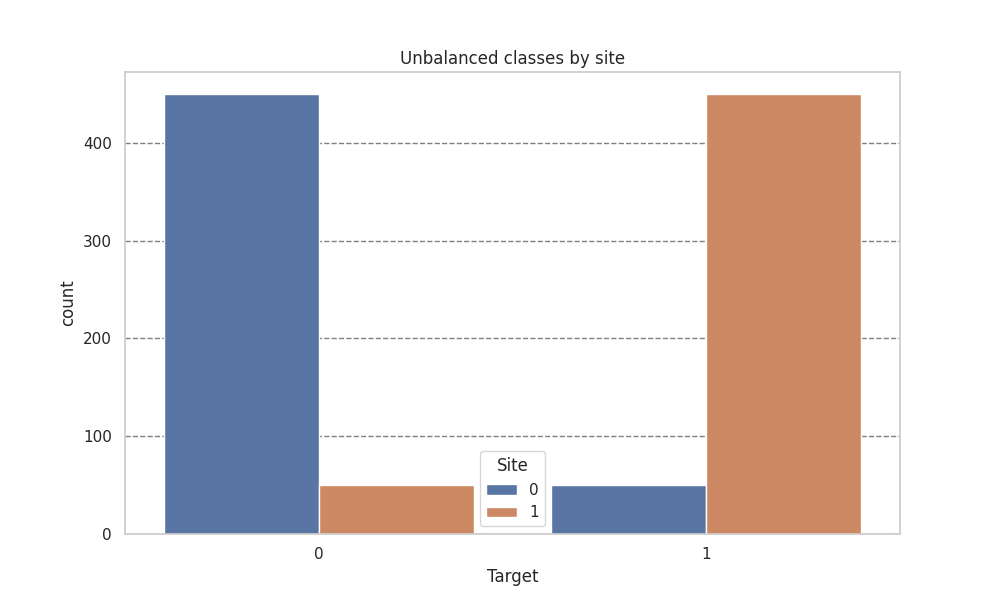
Analysing ComBatGAM behaviour with imbalance across sites

Imports

import matplotlib.pyplot as plt
import pandas as pd
import seaborn as sns

from uniharmony import verbosity
from uniharmony.combat import ComBatGAM
from uniharmony.datasets import make_multisite_classification


sns.set_theme(style="whitegrid")
verbosity("warning")

Data generation

X, y, sites = make_multisite_classification(
    n_features=2,
    signal_strength=2,
    site_effect_strength=0,  # NO site effect
    balance_per_site=[0.1, 0.9],
)
df = pd.DataFrame({"Target": y, "Site": sites})

plt.figure(figsize=[10, 6])
plt.title("Unbalanced classes by site")
sns.countplot(df, x="Target", hue="Site")
plt.grid(axis="y", color="black", alpha=0.5, linestyle="--")

Caution

Note that we are harmonising the whole dataset, which must be avoided in ML scenarios. This is just to illustrate the effect of harmonisation.

Harmonisation

combat = ComBatGAM()
combat.fit(X.copy(), sites, smooth_covariates=y.reshape(-1, 1))
X_harmonized = combat.transform(X, sites, smooth_covariates=y.reshape(-1, 1))

Plotting

df_orig = pd.DataFrame(X, columns=["Feature1", "Feature2"])
df_orig["Site"] = sites
df_orig["Target"] = y
df_orig["Phase"] = "Original"

df_harm = pd.DataFrame(X_harmonized, columns=["Feature1", "Feature2"])
df_harm["Site"] = sites
df_harm["Target"] = y
df_harm["Phase"] = "Harmonized"


fig, axes = plt.subplots(1, 2, figsize=(12, 5), sharex=True, sharey=True)
sns.scatterplot(data=df_orig, x="Feature1", y="Feature2", hue="Target", alpha=0.6, ax=axes[0])
axes[0].set_title("Original data by site")
axes[0].grid(alpha=0.3, color="black", linestyle="--")

sns.scatterplot(data=df_harm, x="Feature1", y="Feature2", hue="Target", alpha=0.6, ax=axes[1])
axes[1].set_title("Harmonized data by site")
axes[1].grid(alpha=0.3, color="black", linestyle="--")
plt.tight_layout()

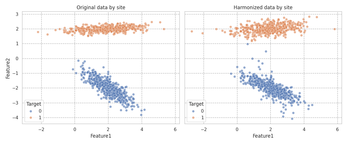
Preserving the target as covariate

Caution

This is also wrong in ML context, where you don’t have access to the full dataset but may be a good option for statistical analysis.

combat = ComBatGAM()
# This is the key line: we need to include the target variable as a covariate
# to preserve its relationship with the features during harmonization.

combat.fit(X.copy(), sites, smooth_covariates=y.reshape(-1, 1))
X_harmonized = combat.transform(X.copy(), sites, smooth_covariates=y.reshape(-1, 1))

df_orig = pd.DataFrame(X, columns=["Feature1", "Feature2"])
df_orig["Site"] = sites
df_orig["Target"] = y

df_orig["Phase"] = "Original"

df_harm = pd.DataFrame(X_harmonized, columns=["Feature1", "Feature2"])
df_harm["Site"] = sites
df_harm["Target"] = y

df_harm["Phase"] = "Harmonized"

Plotting

# Plot data distribution by site before and after harmonisation
fig, axes = plt.subplots(1, 2, figsize=(12, 5), sharex=True, sharey=True)
sns.scatterplot(data=df_orig, x="Feature1", y="Feature2", hue="Site", alpha=0.6, ax=axes[0])
axes[0].set_title("Original data by site")
sns.scatterplot(data=df_harm, x="Feature1", y="Feature2", hue="Site", alpha=0.6, ax=axes[1])
axes[1].set_title("Harmonized data by site")
plt.tight_layout()

Take-home message

ComBatGAM cannot preserve the target variance in class imbalance scenarios unless we preserve it as covariate. Note that preserving the target as covariate may be suited for statistical analysis, but not for ML scenarios. The implementation warns us about the preservation of a covariate.