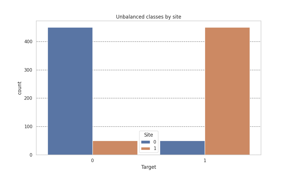
Analyzing NeuroComBat behavior with imbalance across sites

Imports

import matplotlib.pyplot as plt
import pandas as pd
import seaborn as sns
from uniharmony.datasets import make_multisite_classification

from uniharmony import verbosity
verbosity("warning")
from uniharmony.combat import NeuroComBat

sns.set_theme(style="whitegrid")

Data generation

X, y, sites = make_multisite_classification(
    n_features=2,
    signal_strength=3,
    site_effect_strength=0,  # NO site effect
    balance_per_site=[[0.1, 0.9],[0.9, 0.1]],
    signal_type="blobs",
)
df = pd.DataFrame({"Target": y, "Site": sites})

plt.figure(figsize=[10, 6])
plt.title("Unbalanced classes by site")
sns.countplot(df, x="Target", hue="Site")
plt.grid(axis="y", color="black", alpha=0.5, linestyle="--")

Caution

Note that we are harmonizing the whole dataset, which must be avoided in ML scenarios. This is just to illustrate the effect of harmonization.

Harmonization

X_harmonized = X.copy()
combat = NeuroComBat()
combat.fit(X_harmonized, sites)
X_harmonized = combat.transform(X_harmonized, sites)

Plotting

df_orig = pd.DataFrame(X, columns=["Feature1", "Feature2"])
df_orig["Site"] = sites
df_orig["Target"] = y
df_orig["Phase"] = "Original"

df_harm = pd.DataFrame(X_harmonized, columns=["Feature1", "Feature2"])
df_harm["Site"] = sites
df_harm["Target"] = y
df_harm["Phase"] = "Harmonized"


fig, axes = plt.subplots(1, 2, figsize=(12, 5), sharex=True, sharey=True)
sns.scatterplot(data=df_orig, x="Feature1", y="Feature2", hue="Site",style="Target", alpha=0.6, ax=axes[0])
axes[0].set_title("Original data by site")
axes[0].grid(alpha=0.3, color="black", linestyle="--")

sns.scatterplot(data=df_harm, x="Feature1", y="Feature2", hue="Site",style="Target", alpha=0.6, ax=axes[1])
axes[1].set_title("Harmonized data by site")
axes[1].grid(alpha=0.3, color="black", linestyle="--")
plt.tight_layout()

import numpy as np

np.array_equal(X, X_harmonized)

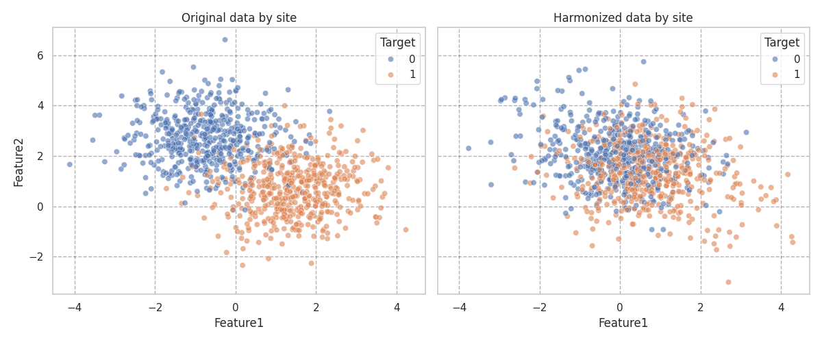
False

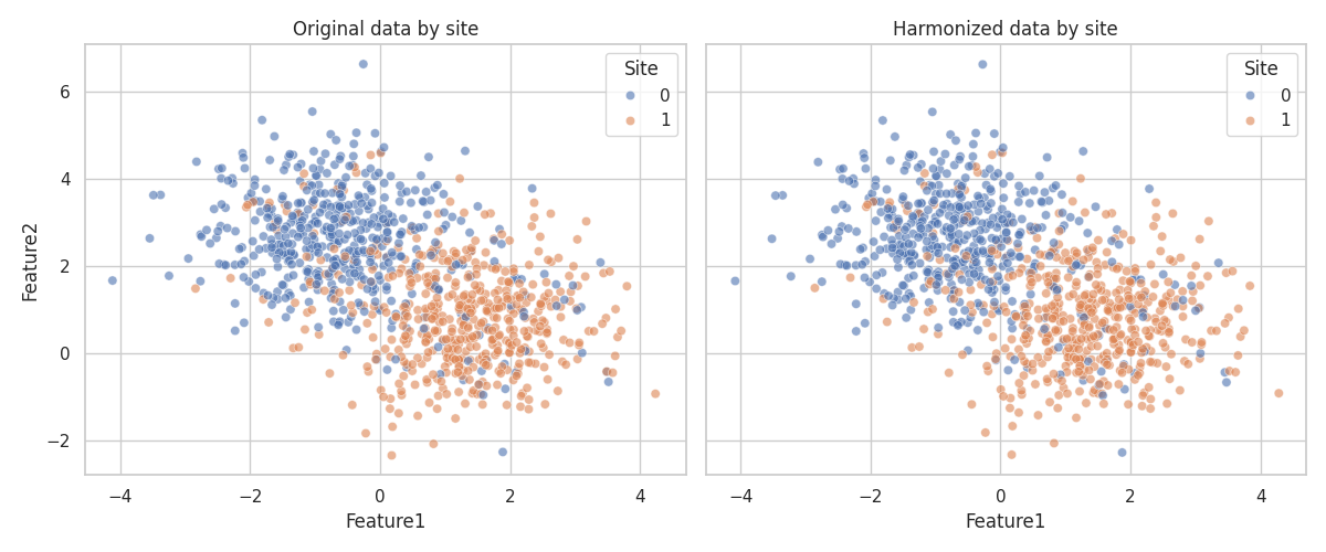
Preserving the target as covariate

Caution

This is also wrong in ML context, where you don’t have access to the full dataset but may be a good option for statistical analysis.

combat = NeuroComBat()
# This is the key line: we need to include the target variable as a covariate
# to preserve its relationship with the features during harmonization.

combat.fit(X, sites, categorical_covariates=y)
X_harmonized = combat.transform(X, sites, categorical_covariates=y)

df_orig = pd.DataFrame(X, columns=["Feature1", "Feature2"])
df_orig["Site"] = sites
df_orig["Target"] = y

df_orig["Phase"] = "Original"

df_harm = pd.DataFrame(X_harmonized, columns=["Feature1", "Feature2"])
df_harm["Site"] = sites
df_harm["Target"] = y

df_harm["Phase"] = "Harmonized"

2026-06-10 10:31:22 [warning  ] You specified categorical and/or continuous covariates to be preserved. If you intend to build a machine learning (ML) model,then make sure that you DO *NOT* preserve the ML model's target as covariate. You will be required to provide the covariate also at transform time, and this will produce data leakage. If you are performing a statistical analysis and want to preserve a variable of interest, then it is correct to specify it as covariate.

Plotting

# Plot data distribution by site before and after harmonization
fig, axes = plt.subplots(1, 2, figsize=(12, 5), sharex=True, sharey=True)
sns.scatterplot(data=df_orig, x="Feature1", y="Feature2", hue="Site", style="Target", alpha=0.6, ax=axes[0])
axes[0].set_title("Original data by site")
sns.scatterplot(data=df_harm, x="Feature1", y="Feature2", hue="Site", style="Target",alpha=0.6, ax=axes[1])
axes[1].set_title("Harmonized data by site")
plt.tight_layout()

Take-home message

ComBat cannot preserve the target variance in class imbalance scenarios unless we preserve it as covariate. Note that preserving the target as covariate may be suited for statistical analysis, but not for ML scenarios. The implementation warns us about the preservation of a covariate.