Note
Go to the end to download the full example code.
Characterise a multisite problem with MAREoS#
Imports#
import matplotlib.pyplot as plt
import pandas as pd
import seaborn as sns
from sklearn.manifold import TSNE

from uniharmony import verbosity
from uniharmony.datasets import load_MAREoS
from uniharmony.plot import plot_2d_components_by_value, plot_2d_projection


sns.set_theme(style="whitegrid")
verbosity("warning")
Data generation#
Let’s load the MAREoS datasets, which simulates several datasets with and without Effects of Site (EoS)
Downloading file 'public_datasets.zip' from 'https://www.imardgroup.com/mareos-benchmark/public_datasets.zip' to '/home/runner/.cache/uniharmony'.

  0%|                                              | 0.00/3.66M [00:00<?, ?B/s]
  1%|▎                                     | 32.8k/3.66M [00:00<00:14, 253kB/s]
  5%|█▊                                     | 176k/3.66M [00:00<00:04, 746kB/s]
 12%|████▌                                 | 440k/3.66M [00:00<00:02, 1.32MB/s]
 23%|████████▋                             | 841k/3.66M [00:00<00:01, 2.14MB/s]
 42%|███████████████▌                     | 1.54M/3.66M [00:00<00:00, 3.32MB/s]
 76%|███████████████████████████▉         | 2.77M/3.66M [00:00<00:00, 5.42MB/s]
  0%|                                              | 0.00/3.66M [00:00<?, ?B/s]
100%|█████████████████████████████████████| 3.66M/3.66M [00:00<00:00, 15.2GB/s]
Unzipping contents of '/home/runner/.cache/uniharmony/public_datasets.zip' to '/home/runner/.cache/uniharmony/MAREoS'
dict_keys(['eos_simple1', 'eos_simple2', 'eos_interaction1', 'eos_interaction2', 'true_simple1', 'true_simple2', 'true_interaction1', 'true_interaction2'])
Now let’s play with tSNE and the plotting helper functions
# EoS signal
dataset = datasets["eos_simple1"]
X = dataset["X"]
y = dataset["y"]
sites = dataset["sites"]
tsne = TSNE(n_components=2, random_state=42, perplexity=30, max_iter=1000, learning_rate="auto")
X_tsne = tsne.fit_transform(X)
tsne_df_eos = pd.DataFrame({"comp1": X_tsne[:, 0], "comp2": X_tsne[:, 1], "site": sites, "target": y})

# True signal
dataset = datasets["true_simple1"]
X = dataset["X"]
y = dataset["y"]
sites = dataset["sites"]
tsne = TSNE(n_components=2, random_state=42, perplexity=30, max_iter=1000, learning_rate="auto")
X_tsne = tsne.fit_transform(X)
tsne_df_true = pd.DataFrame({"comp1": X_tsne[:, 0], "comp2": X_tsne[:, 1], "site": sites, "target": y})

# Initialize figure
fig, axes = plt.subplots(2, 2, figsize=(16, 14))

# Plot 1: EoS By site
ax1 = axes[0, 0]
plot_2d_components_by_value(tsne_df_eos, "site", "tSNE", ax1)

# Plot 2: EoS By target
ax2 = axes[1, 0]
plot_2d_components_by_value(tsne_df_eos, "target", "tSNE", ax2)

# # Plot 3: True Signal By site
ax3 = axes[0, 1]
plot_2d_components_by_value(tsne_df_true, "site", "tSNE", ax3)

# Plot 4: True Signal By target
ax4 = axes[1, 1]
plot_2d_components_by_value(tsne_df_true, "target", "tSNE", ax4)
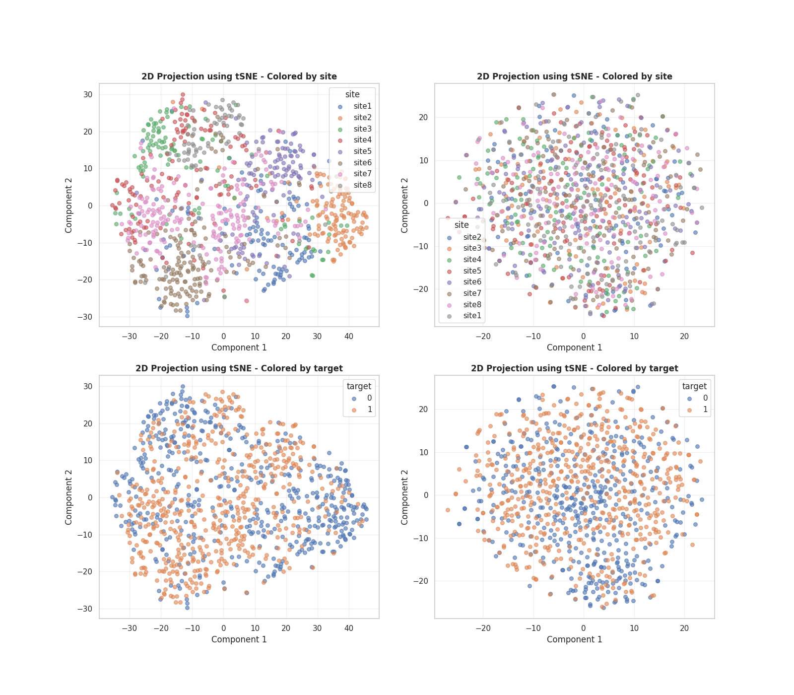
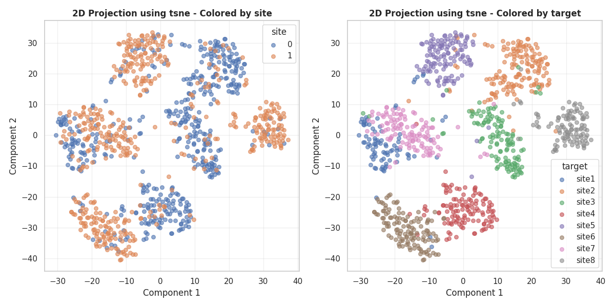
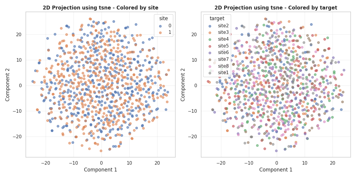
We see that, for the EoS signal, the main tSNE components are related with the sites, which are also realted with the targets. On the other hand, there is not a clear relationship between the sites nor the target for the True signal.
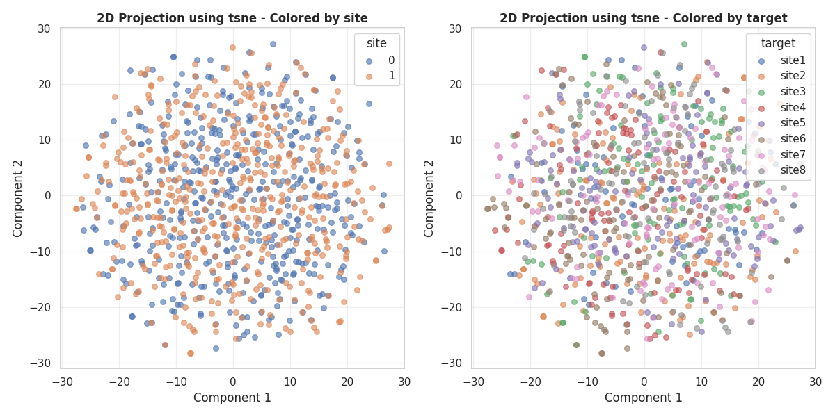
Now let’s use the plot_tsne funtion which can simplify the code and will allowd us a fast and simple exploration

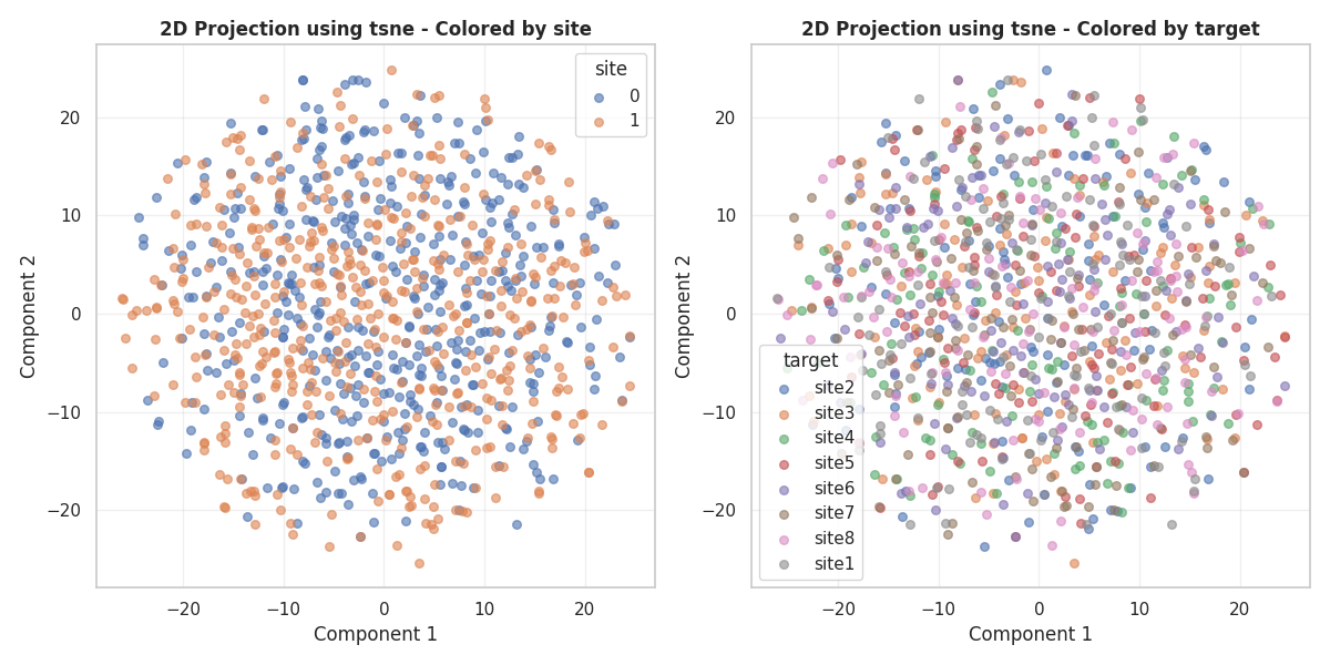
(<Figure size 1200x600 with 2 Axes>, array([<Axes: title={'center': '2D Projection using tsne - Colored by site'}, xlabel='Component 1', ylabel='Component 2'>,
       <Axes: title={'center': '2D Projection using tsne - Colored by target'}, xlabel='Component 1', ylabel='Component 2'>],
      dtype=object))
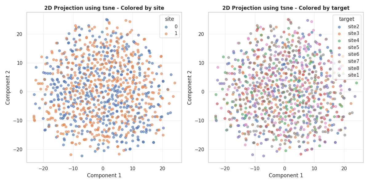
Total running time of the script: (0 minutes 59.838 seconds)