Explore EoS with dimensionality reduction techniques

The first step before applying any harmonization technique is to understand and characterize our data.

Usually, we deal with high dimensional data. In order to reduce the dimensions of the problem and see how much target and Effect of Site (EoS) information there is in our data.

Let’s explore how simulated data looks like using different dimensionality reduction methods.

For this we will use the function plot_2d_projection of uniharmony, that allows us to pass our data and automatically generate a scatter plot.

Imports

import matplotlib.pyplot as plt
import seaborn as sns
from sklearn.decomposition import FastICA

from uniharmony import verbosity
from uniharmony.datasets import make_multisite_classification
from uniharmony.plot import plot_2d_projection


sns.set_theme(style="whitegrid")
verbosity("warning")

Data generation

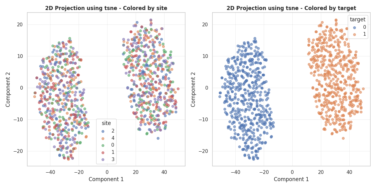
Let’s simulate data with only Effects of Site (EoS) or only real signal, and see how tSNE groups the target and Eos.

X, y, sites = make_multisite_classification(n_sites=5, signal_strength=10, site_effect_strength=0)
# Using the function as default. The function will use t-SNE as default dimensionality reductor.
plot_2d_projection(X, sites, y)

(<Figure size 1200x600 with 2 Axes>, array([<Axes: title={'center': '2D Projection using tsne - Colored by site'}, xlabel='Component 1', ylabel='Component 2'>,
       <Axes: title={'center': '2D Projection using tsne - Colored by target'}, xlabel='Component 1', ylabel='Component 2'>],
      dtype=object))

X, y, sites = make_multisite_classification(n_sites=5, signal_strength=0, site_effect_strength=10, random_state=23)
plot_2d_projection(X, sites, y)
plt.show()

2026-05-18 13:03:39 [warning  ] signal_strength is 0. Adding a delta (1e-6) to signal_strength to avoid degenerate data.

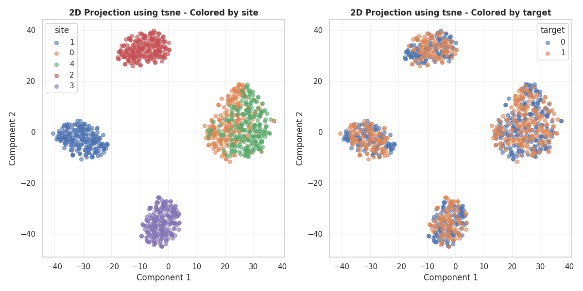
In the first plot, we see that classes are perfectly separated and the sites are all mixed in the clusters. This is because tSNE used the target information to get the clusters, as there was no EoS information.

In the second plot, exactly the opposite happened, tSNE clustered the sites almost perfectly.

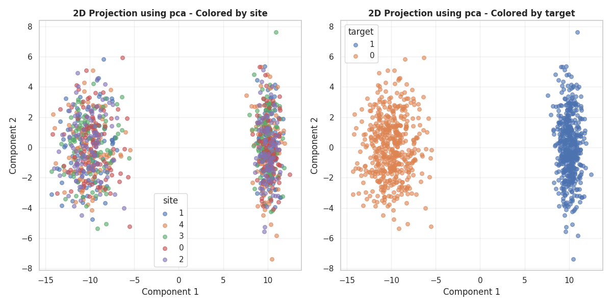
Let’s try now another dimensionality reduction method.

X, y, sites = make_multisite_classification(n_classes=2, n_sites=5, n_features=1200, signal_strength=10, site_effect_strength=0)
# We can also pass the method as string. Only a few methods are available to pass as string in "method"
plot_2d_projection(X, sites, y, method="pca")

(<Figure size 1200x600 with 2 Axes>, array([<Axes: title={'center': '2D Projection using pca - Colored by site'}, xlabel='Component 1', ylabel='Component 2'>,
       <Axes: title={'center': '2D Projection using pca - Colored by target'}, xlabel='Component 1', ylabel='Component 2'>],
      dtype=object))

X, y, sites = make_multisite_classification(n_classes=2, n_sites=5, n_features=120, signal_strength=0, site_effect_strength=10)
fig, axes = plot_2d_projection(X, sites, y, method="pca")
plt.show()

2026-05-18 13:03:44 [warning  ] signal_strength is 0. Adding a delta (1e-6) to signal_strength to avoid degenerate data.

Dimensionality reduction

dim_reductor = FastICA(n_components=2)
X, y, sites = make_multisite_classification(n_classes=2, n_sites=5, n_features=1200, signal_strength=10, site_effect_strength=0)
# We can also pass directly an instance of the dimensionality reductor that we want to use.
plot_2d_projection(X, sites, y, dim_reductor=dim_reductor)

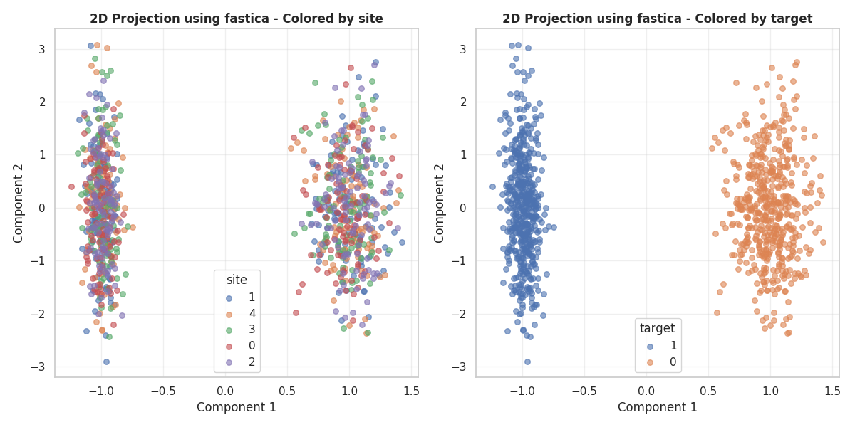
(<Figure size 1200x600 with 2 Axes>, array([<Axes: title={'center': '2D Projection using fastica - Colored by site'}, xlabel='Component 1', ylabel='Component 2'>,
       <Axes: title={'center': '2D Projection using fastica - Colored by target'}, xlabel='Component 1', ylabel='Component 2'>],
      dtype=object))

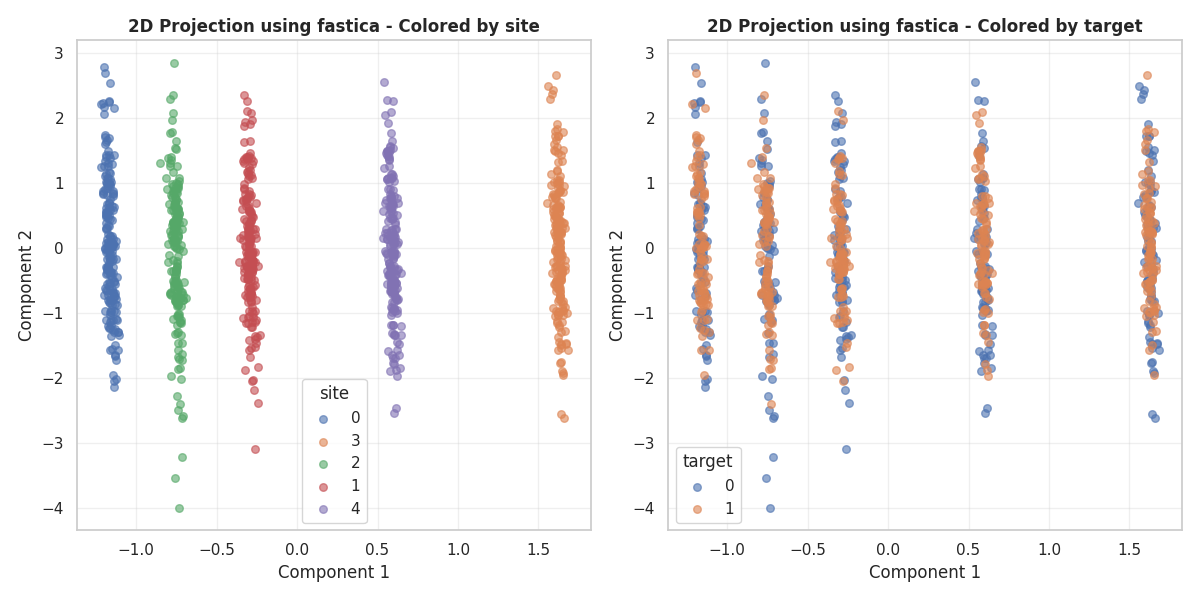
X, y, sites = make_multisite_classification(n_classes=2, n_sites=5, n_features=120, signal_strength=0, site_effect_strength=10)
fig, axes = plot_2d_projection(X, sites, y, dim_reductor=dim_reductor)
plt.show()

2026-05-18 13:03:46 [warning  ] signal_strength is 0. Adding a delta (1e-6) to signal_strength to avoid degenerate data.

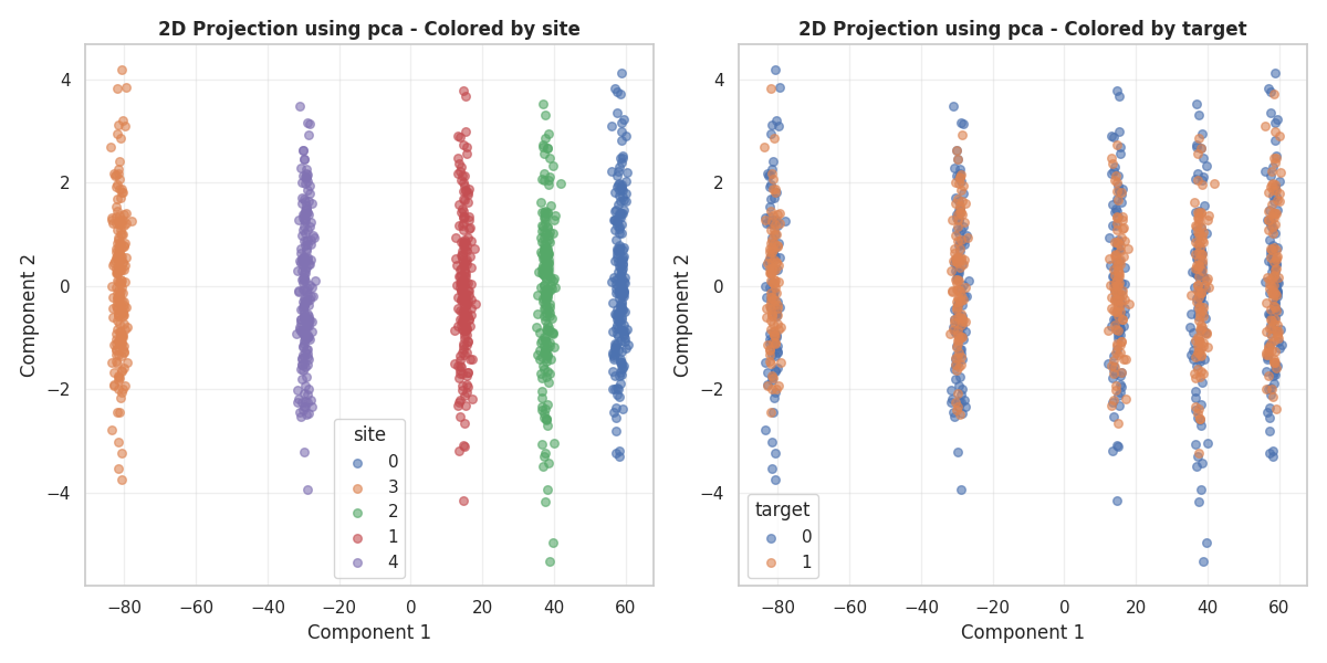
We found similar behavior using PCA os FastICA, but different clusters were generated.